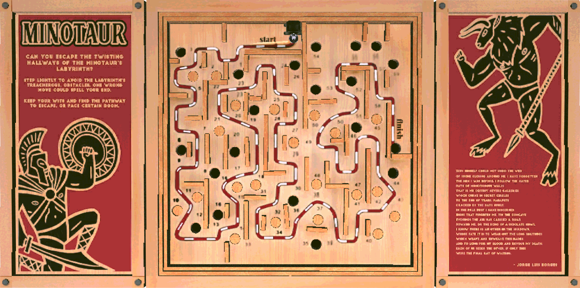
What is Minotaur?
Minotaur (2020) served as a pilot project for developing ClowderBridge, a plugin that synchronizes data between Unity and Clowder. Clowder is an open-source data storage and analytics tool designed to facilitate data collection and management. The game was released on Desktop, Mobile AR, and Web platforms, all of which contributed to a shared dataset.
Inspired by BRIO's Labyrinth (1946), Minotaur incorporates additional tracking parameters, such as "cheats" when players deviate from the dashed line to take shortcuts. To alleviate player frustration, Medium and Easy modes were introduced, which block half and all holes, respectively.
Gameplay
Analysis
As an exercise in data analytics and datamining, we made sure to capture as much of a complete picture of each gameplay session as possible.
Each log contains an identity node which says what platform the game was played on, the session difficulty, the control style.
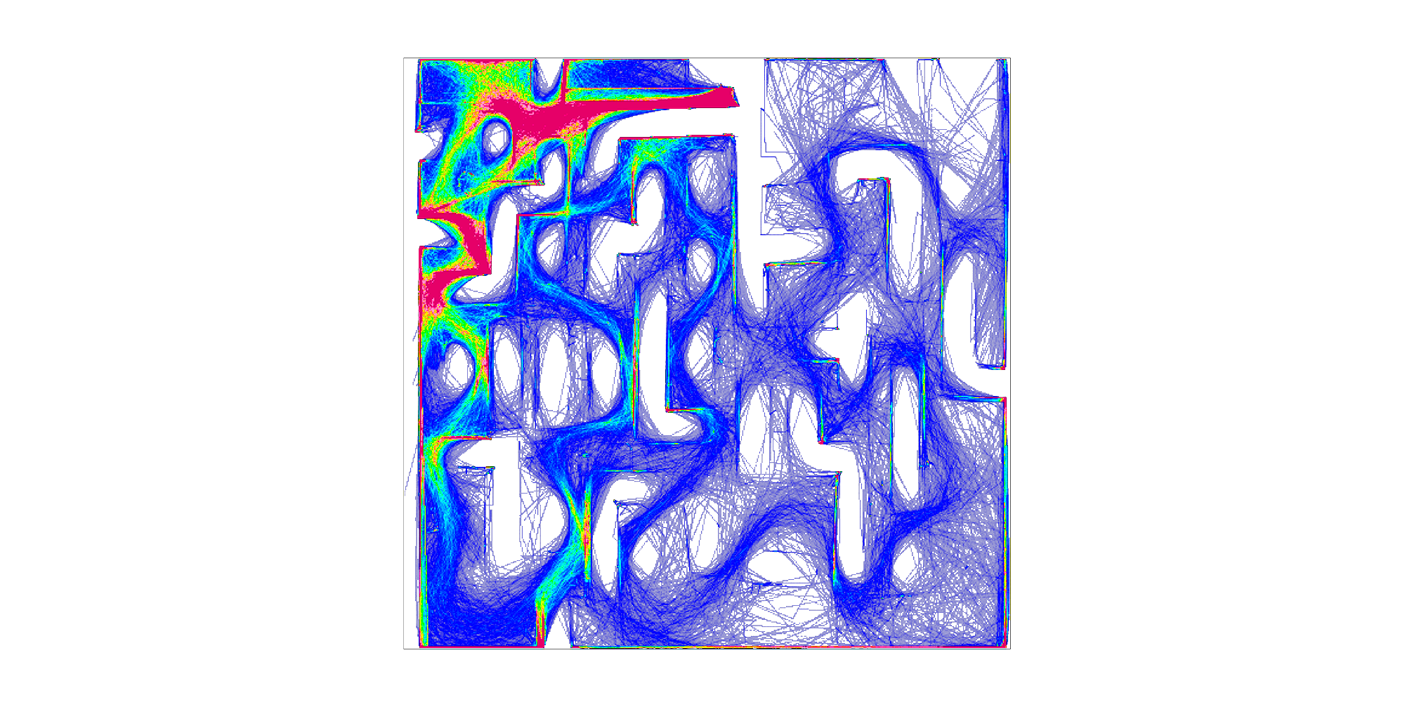
After the preamble, we log the position of the ball every half second.
The last part of the log is for events, where each object is an announcement (like hit hole, cheated, won), as well as a set of additional metadata to help make sense of the event later, eg. where the event happened and the time.
The analyses below are attempts to draw insight from the ~5000 recorded runs, answering basic questions like:
- Which holes were the most tricky? What is characteristic of tricky holes?
- Which shortcuts were the most common?
- How can we balance the penalty for cheats such that top runs for no-cheat and cheat runs have similar scores?
- How can we develop a session grading system based on the real-world performance of players?
Which Holes were Hardest? (Advanced Difficulty)
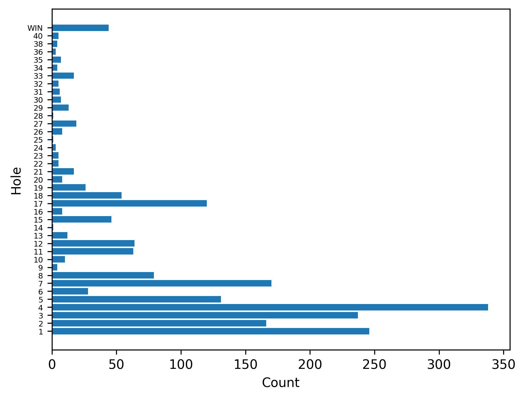
We start by counting the number of players that fell into each hole. We only look at advanced difficulty sessions as easier difficulties remove holes from the board, making the data incomparable.
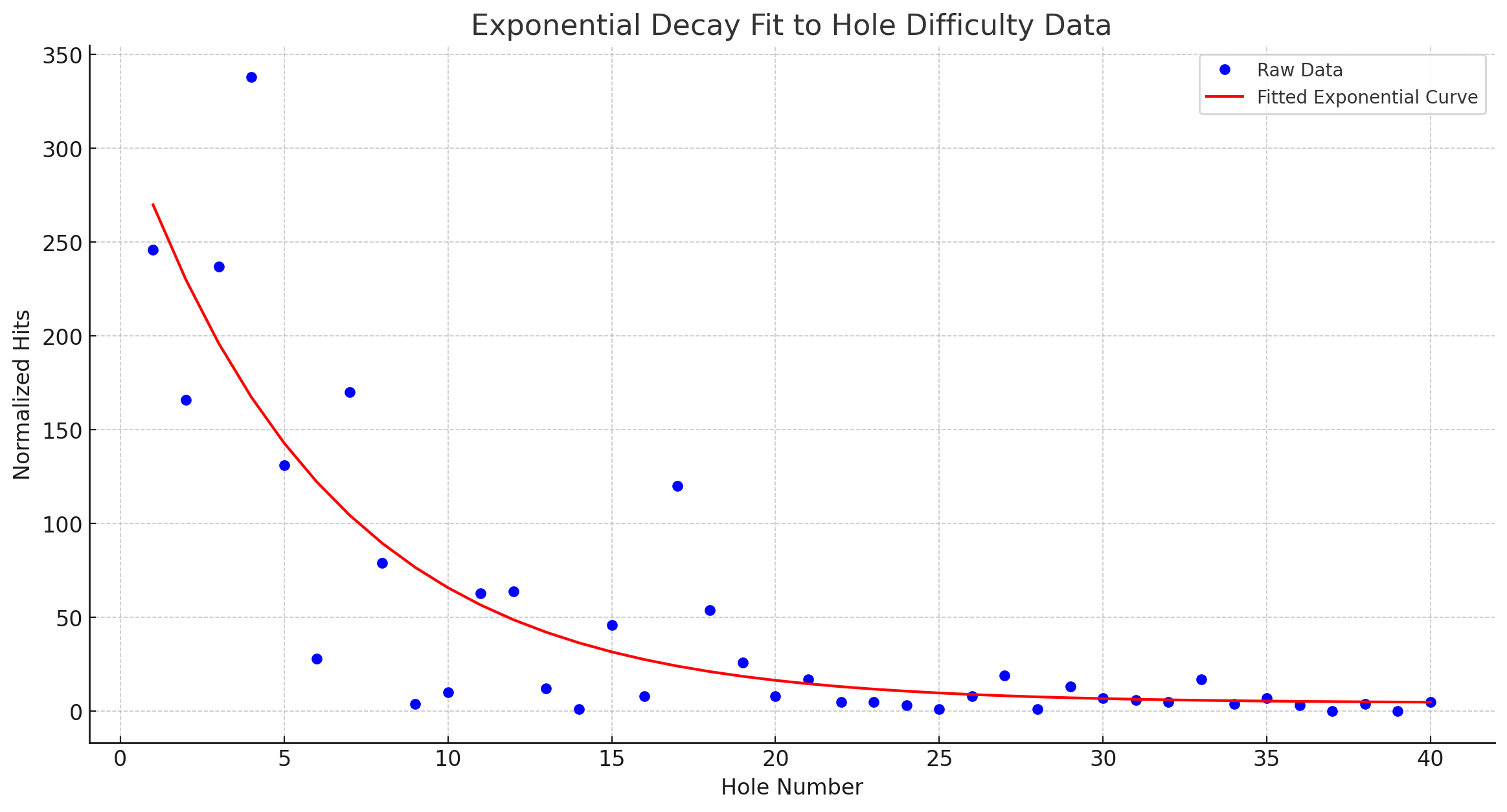
To assess the relative difficulty of each hole, we start by fitting an exponential curve to our observed data. Since each hole is encountered sequentially and players 'fall out' before reaching later holes, we can expect the powerlaw effect we see. With the exponential curve fit, we can express the relative difficulty of each hole as the residual between how many players we'd expect to fall down it based on its proximity to the start, and how many were actually observed to fall down it.
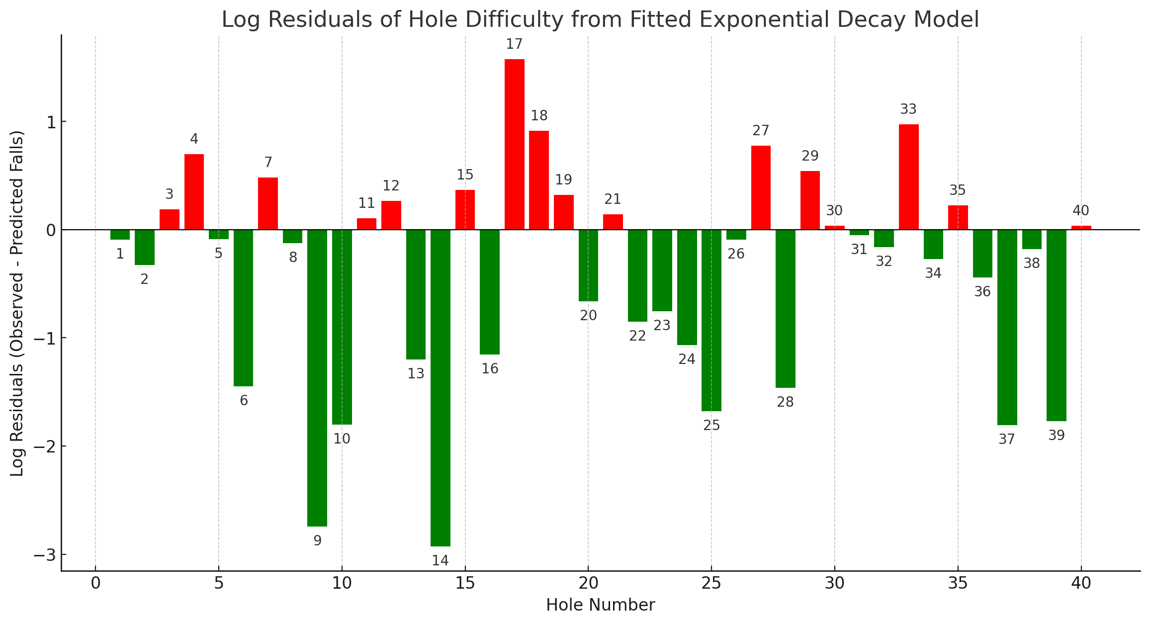
The final figure above characterizes each hole as being more or less difficult than expected.
Upward bars are harder than expected, downward are easier than expected.
We visualize the residuals between observed falls and the exponential model in a logarithmic format. This transformation is particularly effective for contrasting the frequency of falls against the exponential expectation, accentuating discrepancies on a multiplicative scale.
The figure at the top of the page has a dropdown to see the difficulties mapped to holes in the maze.
One observation from the analysis is that the most difficult holes share a common design feature. This challenge sequence requires the player to (1) not slide along a wall, (2) accelerate toward a hole, and then (3) maneuver around it. Such a combination is one of the most significant challenges for this kind of marble maze.
Cheat Penalty Balancing
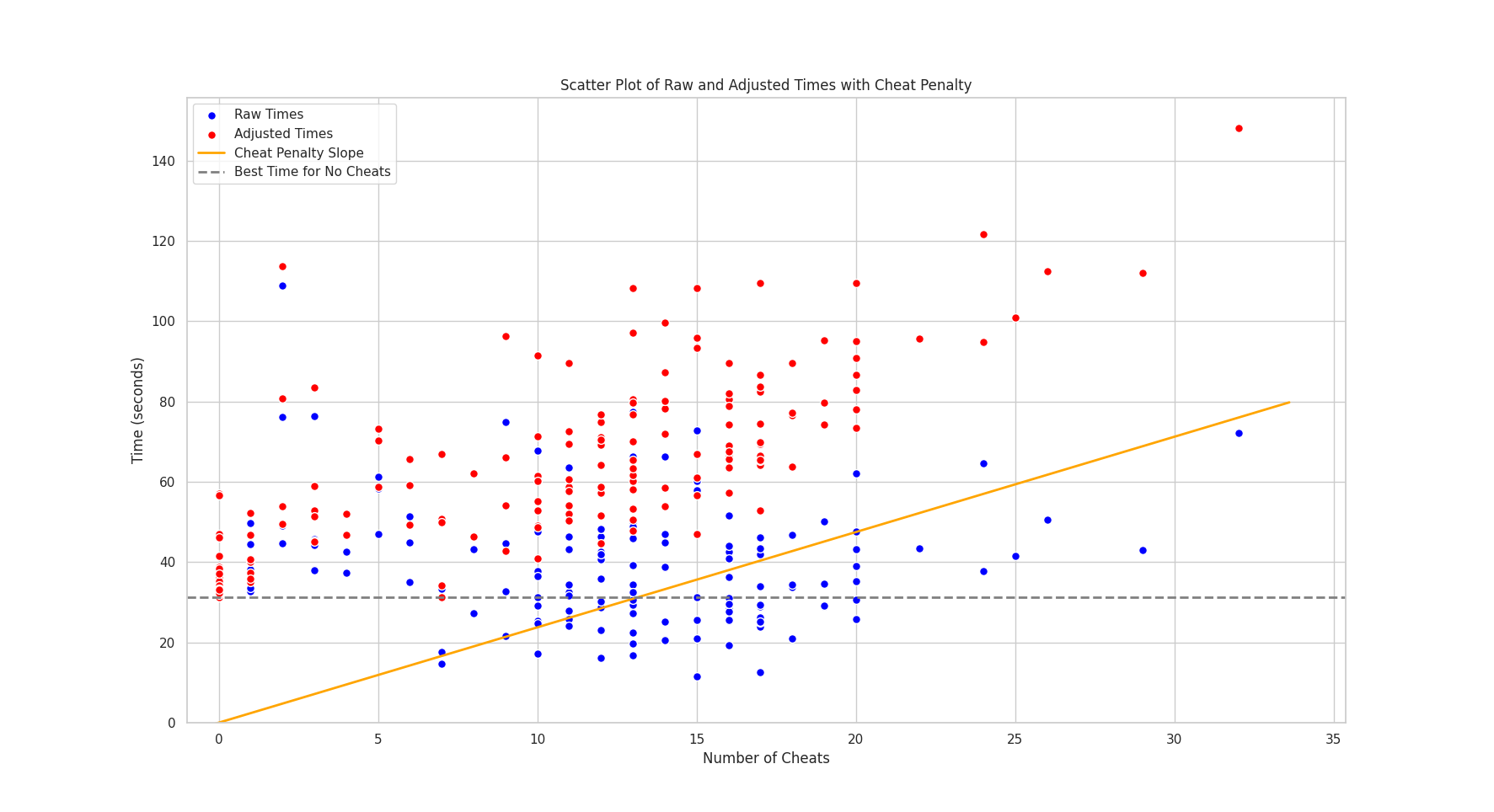
In Minotaur, players can cheat by taking shortcuts through the maze. There's a visualization of which shortcuts were used as a dropdown option in the top visualization. Cheating creates new challenges for the player as the board shakes in response, but is a strategies for getting even lower times. Our initial approach to penalizing cheats was straightforward: a flat 15-second addition to the player's time per cheat. However, analysis showed this might have been too severe based on the best times that cheating would allow. The analysis below follows how we'd adjust the time penalty to bring the best cheat scores in line with the best no-cheat scores based on the collected data.
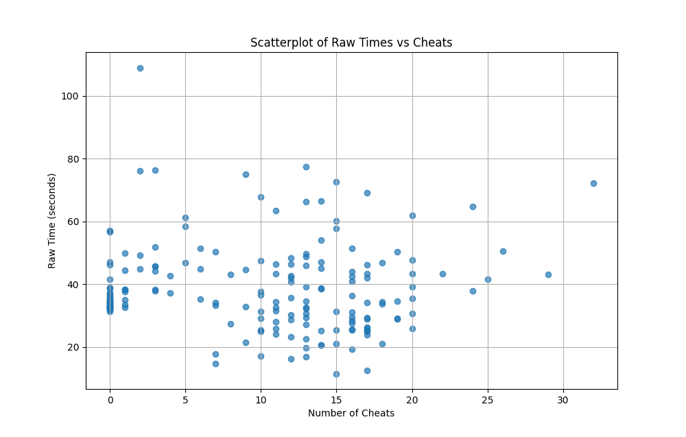
First, we performed a scatterplot of raw times to complete along with cheat counts (below). We can see that many cheat runs took longer than no-cheat runs. A few were much faster. No-cheat runs actually show a much tighter distribution of performance, possibly showing a behavior characteristic of noncheaters.
We wondered how representative this 'completed runs' dataset actually was of our player population. Since scores are user submitted (non-random), we might have a skewed distribution where highly engaged players submit far more runs than the average player. This is a common phenomenon in many user-generated datasets, often referred to as the Pareto principle or the "80/20 rule."
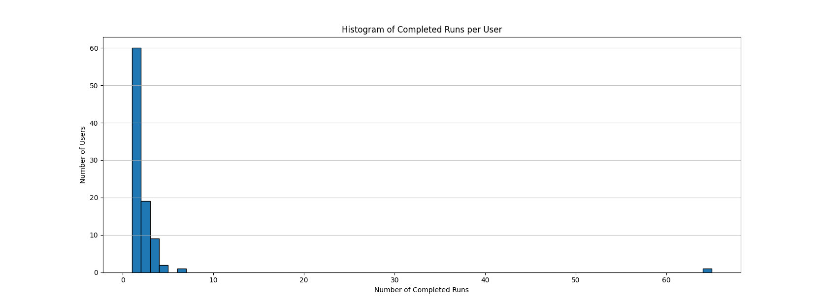
The histogram above confirms a small number of highly engaged players produced a similar amount of data as the rest of the cohort combined. In games with larger playerbases, it becomes productive to bucket these distinct subpopulations and tune scores for each of them separately, such as 'competitive' vs 'casual' players. However, we will continue to run our analysis with the full dataset rather than binning as it's just an exercise. We might consider strategies for binning casual vs competitive players as future work.
Further examination involved a detailed look at the first quartile times across cheat counts, represented in a series of boxplots. Our analysis indicated that there's no linear relationship in the data between number of cheats and time, as shown in the following graph. Cheating only becomes a significant net-positive stategy for overall time between 7 and 22.
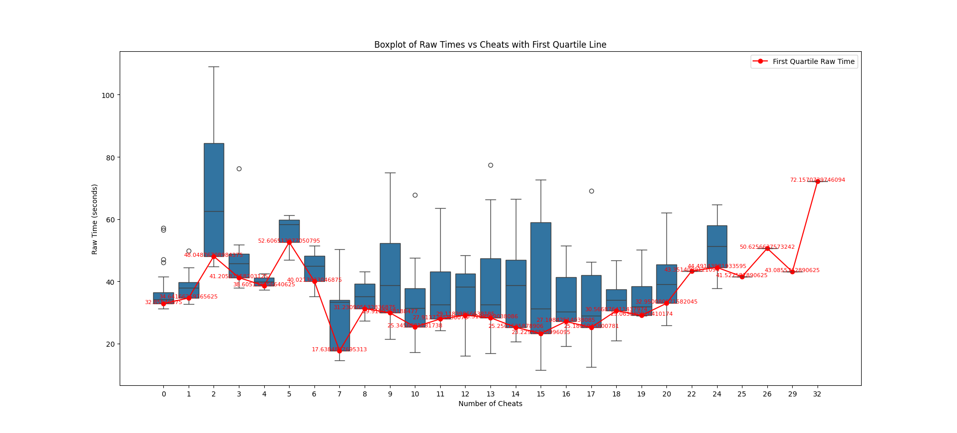
To figure out a proper cheat penalty, we decided to instead focus on outliers. We find the largest negative slope between the best non-cheat run and the best cheat run. The inverted (positive) version of this slope becomes an easy to understand cheat penalty. When applied, it brings all best cheat times in line with the best non-cheat times. After running a solver to find the slope, we reduced the penalty to 2.3 seconds per cheat. The final scatterplot with adjusted times, seen below, demonstrates the effectiveness of this simple approach.
Through this data-driven approach, we have established a cheat penalty that upholds the competitive spirit of the game while acknowledging the strategic use of cheats by some players.
Establishing a Data-Driven Grading System
When players complete a maze run, they recieve a grade based on their time. Originally, these grades were determined by a handful of runs during development. The data collected shows players quickly surprassed these scores, meaning most were considered S++.
We show how we would update the grading criteria based on the completed runs collected so far, based on the distribution of times across completed runs, much like classwork. The completion times are rather compact in the dataset, meaning the grades are sensitive to second increments.
| Grade | Time (seconds) | Distribution Cut |
|---|---|---|
| S++ | < 30.20 | Top Performers (Beyond current best) |
| A+ | < 32.22 | 90-100th percentile |
| A | ≥ 32.22 and < 32.45 | 80-90th percentile |
| B | ≥ 32.45 and < 33.36 | 60-80th percentile |
| C | ≥ 33.36 and < 34.67 | 40-60th percentile |
| D | ≥ 34.67 and < 37.17 | 20-40th percentile |
| F | ≥ 37.17 | Below 20th percentile |
Refining the Grading System
In response to the observed Pareto distribution in our winning-runs dataset—where a few prolific players dominated the completed runs—we've implemented a data normalization strategy. To foster a more representative dataset without binning user-types, we've capped the contribution of any single player to five winning sessions, randomly sampled if they have more. This adjustment curtails the overrepresentation of frequent players and ensures our grading system more accurately reflects the broader gaming community, hopefully providing a more forgiving grade scale while still motivating new and better times.
| Grade | Time (seconds) | Distribution Cut |
|---|---|---|
| S++ | < 30.00 | Exceptional (Beyond current best) |
| S+ | < 31.00 | Elite (Top performers) |
| S | < 32.00 | Excellent |
| A+ | < 33.45 | 90-100th percentile |
| A | ≥ 33.45 and < 34.55 | 80-90th percentile |
| B | ≥ 34.55 and < 35.72 | 60-80th percentile |
| C | ≥ 35.72 and < 37.22 | 40-60th percentile |
| D | ≥ 37.22 and < 42.52 | 20-40th percentile |
| F | ≥ 42.52 | Below 20th percentile |
The impact of this change can be observed through an example: a raw time of 30 seconds with 5 cheats previously adjusted to 41.87 seconds. Under the new system, the adjusted time is 42.69 seconds, which corresponds to a different grade, reflecting our more representative and balanced grading criteria.
Credits
-
Colter Wehmeier
Development, Analysis
-
Azurite Coast
Music http://azuritecoast.bandcamp.com
-
Scott Cotterell
Graphic Design @skcotterell